Examples

Reference Manual Example

In this section we solve how to define and solve the example given at the beginning of the GLPK C API reference manual.

\[\begin{split}\begin{aligned} & \underset{\mathbf{x}}{\text{maximize}} & & Z = 10 x_0 + 6 x_1 + 4 x_2 & \\ & \text{subject to} & & p = x_0 + x_1 + x_2 & \\ & & & q = 10 x_0 + 4 x_1 + 5 x_2 & \\ & & & r = 2 x_0 + 2 x_1 + 6 x_2 & \\ & \text{and bounds of variables} & & - \infty \lt p \leq 100 & 0 \leq x_0 \lt \infty \\ & & & - \infty \lt q \leq 600 & 0 \leq x_1 \lt \infty \\ & & & - \infty \lt r \leq 300 & 0 \leq x_2 \lt \infty \\ \end{aligned}\end{split}\]

The Implementation

Here is the implementation of that linear program within PyGLPK:

import glpk                         # Import the GLPK module

lp = glpk.LPX()                     # Create empty problem instance
lp.name = 'sample'                  # Assign symbolic name to problem
lp.obj.maximize = True              # Set this as a maximization problem
lp.rows.add(3)                      # Append three rows to this instance
for r in lp.rows:                   # Iterate over all rows
    r.name = chr(ord('p')+r.index)  # Name them p, q, and r
lp.rows[0].bounds = None, 100.0     # Set bound -inf < p <= 100
lp.rows[1].bounds = None, 600.0     # Set bound -inf < q <= 600
lp.rows[2].bounds = None, 300.0     # Set bound -inf < r <= 300
lp.cols.add(3)                      # Append three columns to this instance
for c in lp.cols:                   # Iterate over all columns
    c.name = 'x%d' % c.index        # Name them x0, x1, and x2
    c.bounds = 0.0, None            # Set bound 0 <= xi < inf
lp.obj[:] = [10.0, 6.0, 4.0]        # Set objective coefficients
lp.matrix = [
    1.0, 1.0, 1.0,                  # Set nonzero entries of the
    10.0, 4.0, 5.0,                 # constraint matrix. (In this
    2.0, 2.0, 6.0                   # case, all are non-zero.)
]
lp.simplex()                        # Solve this LP with the simplex method
print 'Z = %g;' % lp.obj.value,     # Retrieve and print obj func value
print '; '.join(                    # Print struct variable names and
                                    # primal values
    '%s = %g' % (c.name, c.primal) for c in lp.cols
)

The Explanation

We shall now go over this implementation section by section.

import glpk

First we need the module of course.

lp = glpk.LPX()                     # Create empty problem instance

Here we construct a new linear program object with a call to the LPX constructor.

lp.name = 'sample'                  # Assign symbolic name to problem

Linear program objects have various attributes. One of them is name, which holds a symbolic name for the program. Initially a program has no name, and name correspondingly has the value None. Here we name the program 'sample'. Programs do not necessarily require names, but a user may wish to give a program a name nonetheless.

lp.obj.maximize = True              # Set this as a maximization problem

Linear program objects contain other less trivial attributes. One of the most important is obj, an object representing the linear program’s objective function. In this case, we are assigning lp.obj’s maximize attribute the value True, informing out linear program that we want to maximize our objective function.

lp.rows.add(3)                      # Append three rows to this instance

Another very important component of lp is the rows attribute, holding an object which indexes over the rows of this linear program. In this case, we call the lp.rows method add, telling it to add three rows to the linear program.

for r in lp.rows:                   # Iterate over all rows
    r.name = chr(ord('p')+r.index)  # Name them p, q, and r

The lp.rows object is also used for accessing particular rows. In this case, we are iterating over each row. In the course of this iteration, r holds the first, second, and third row. We want to name these rows 'p', 'q', and 'r', in order.

Note that an individual row is an object in itself. It also has a name attribute, to which we assign the character with ASCII value of p plus whatever the index of this row is. The first row has index of 0, the next 1, the next and last 2. So, this will give us the desired names.

lp.rows[0].bounds = None, 100.0     # Set bound -inf < p <= 100
lp.rows[1].bounds = None, 600.0     # Set bound -inf < q <= 600
lp.rows[2].bounds = None, 300.0     # Set bound -inf < r <= 300

In addition to iterating over all rows, we can access a particular row by indexing the lp.rows object. In this case we index by the numeric row index. (Now that we have set their names, we could alternatively index them by their names!)

In this case, we are using the row’s bounds attribute to set the bounds for the corresponding auxiliary variable. Bounds consist of a lower and upper bound. In this case, we are specifying that we always want the lower end unbounded (by assigning None, indicating no bound in that direction), and otherwise setting an appropriate upper bound.

lp.cols.add(3)                      # Append three columns to this instance

In addition to the rows object, there is also a cols object for creating and accessing columns. Indeed, the two objects have the same type. In this case, we see we are adding three columns to the linear program.

for c in lp.cols:                   # Iterate over all columns
    c.name = 'x%d' % c.index        # Name them x0, x1, and x2
    c.bounds = 0.0, None            # Set bound 0 <= xi < inf

Similar to how we iterated over and assigned names to the rows, in this case we assign appropriate names to our columns. We also assign bounds to each column’s associated structural variable, though in this case we want each structural variable to be greater than 0, and have no upper bound.

lp.obj[:] = [10.0, 6.0, 4.0]        # Set objective coefficients

There is one objective coefficient for every column. In this, we set all the coefficients at once to their desired values. Note that these lp.obj objects act like sequences over the objective coefficient values, just as the row and column collections do over rows and the columns.

lp.matrix = [
    1.0, 1.0, 1.0,                  # Set nonzero entries of the
    10.0, 4.0, 5.0,                 # constraint matrix. (In this
    2.0, 2.0, 6.0                   # case, all are non-zero.)
]

We are setting the non-zero entries of the coefficient constraint matrix by assigning to the linear program’s matrix attribute. Matrix entries are either (1) values, or (2) tuples specifying the row index, column index, and value. In the first case, if it is just a value with the indices omitted, it assumes that the value specified is for the next value in the constraint matrix, read top to bottom, left to right. We could also have explicitly defined the indices with this equivalent statement:

lp.matrix = [
    (0, 0, 1.0), (0, 1, 1.0), (0, 2, 1.0),
    (1, 0, 10.0), (1, 1, 4.0), (1, 2, 5.0),
    (2, 0, 2.0), (2, 1, 2.0), (2, 2, 6.0)
]

But we did not. Let’s move on.

lp.simplex()                        # Solve this LP with the simplex method

Here we are calling a simplex solver to solve the defined linear program!

print 'Z = %g;' % lp.obj.value,     # Retrieve and print obj func value
print '; '.join(                    # Print struct variable names and
                                    # primal values
    '%s = %g' % (c.name, c.primal) for c in lp.cols
)

After optimization, we want to print out the value of the objective function (as stored in lp.obj.value), and the value of the primal variable for each of the columns (as stored in each column’s primal attribute).

This all results in this output.

Z = 733.333; x0 = 33.3333; x1 = 66.6667; x2 = 0

Max Flow Example

In this section we show a simple example of how to use PyGLPK to solve max flow problems.

How to Solve

Suppose we have a directed graph with a source and sink node, and a mapping from edges to maximal flow capacity for that edge. Our goal is to find a maximal feasible flow. This is the maximum flow problem.

This is our strategy of how to solve this with a linear program:

• For each edge, we define a structural variable (a column). The primal value of this structural variable is the flow assigned to the corresponding edge. We constrain this so it cannot exceed the edge’s capacity.

• We define our objective function as the net flow of the source, a quantity we wish to maximize.

• For each non-source and non-sink node, we must have 0 net flow. So, for each non-source/sink node, we define an auxiliary variable (a row) equal to the sum of flows in minus the sum of flows out, which we constrain to be 0.

• We run the solver, and return the assignment of edges to flows.

For the purpose of our function, we encode our capacity graph as a list of three element tuples. Each tuple consists of a from node, a to node, and a capacity of the conduit from the from to the to node. Nodes can be anything Python can hash.

The function accepts such a capacity graph, and returns the a similar list of three element tuples. The list is identical as the input list, except the capacities are replaced with the assigned flow.

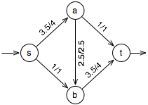
In the example graph seen at right (with given assigned/capacity weights given for the nodes), we have a source and sink 's' and 't', and other nodes 'a' and 'b'. We would represent this capacity graph as [('s','a',4), ('s','b',1), ('a','b',2.5), ('a','t',1), ('b','t',4)]

The Implementation

Here is the implementation of that function:

import glpk


def maxflow(capgraph, s, t):
    # map non-source/sink nodes to row num
    node2rnum = {}
    for nfrom, nto, cap in capgraph:
        if nfrom != s and nfrom != t:
            node2rnum.setdefault(nfrom, len(node2rnum))
        if nto != s and nto != t:
            node2rnum.setdefault(nto, len(node2rnum))

    # empty LP instance
    lp = glpk.LPX()

    # stop annoying messages
    glpk.env.term_on = False

    # as many columns cap-graph edges
    lp.cols.add(len(capgraph))
    # as many rows as non-source/sink nodes
    lp.rows.add(len(node2rnum))

    # net flow for non-source/sink is 0
    for row in lp.rows:
        row.bounds = 0

    # will hold constraint matrix entries
    mat = []

    for colnum, (nfrom, nto, cap) in enumerate(capgraph):
        # flow along edge bounded by capacity
        lp.cols[colnum].bounds = 0, cap

        if nfrom == s:
            # flow from source increases flow value
            lp.obj[colnum] = 1.0
        elif nto == s:
            # flow to source decreases flow value
            lp.obj[colnum] = -1.0

        if nfrom in node2rnum:
            # flow from node decreases its net flow
            mat.append((node2rnum[nfrom], colnum, -1.0))
        if nto in node2rnum:
            # flow to node increases its net flow
            mat.append((node2rnum[nto], colnum, 1.0))

    # want source s max flow maximized
    lp.obj.maximize = True
    # assign 0 net-flow constraint matrix
    lp.matrix = mat

    # this should work unless capgraph bad
    lp.simplex()

    # return edges with assigned flow
    return [
        (nfrom, nto, col.value)
        for col, (nfrom, nto, cap) in zip(lp.cols, capgraph)
    ]

capgraph = [
    ('s', 'a', 4), ('s', 'b', 1),
    ('a', 'b', 2.5), ('a', 't', 1), ('b', 't', 4)
]
print(maxflow(capgraph, 's', 't'))

[('s', 'a', 3.5), ('s', 'b', 1.0), ('a', 'b', 2.5),
 ('a', 't', 1.0), ('b', 't', 3.5)]

The Explanation

We shall now go over this function section by section!

    # map non-source/sink nodes to row num
    node2rnum = {}
    for nfrom, nto, cap in capgraph:
        if nfrom != s and nfrom != t:
            node2rnum.setdefault(nfrom, len(node2rnum))
        if nto != s and nto != t:
            node2rnum.setdefault(nto, len(node2rnum))

This is pure non-PyGLPK code, but it is doing something important for the linear program. Recall that we wanted a row for every non-source/sink node. In order to facilitate this, we first go through the capacity graph and map each node identifier (except the source and sink) to a unique integer, counting from 0 onwards.

    # empty LP instance
    lp = glpk.LPX()

We create an empty LPX instance.

    # stop annoying messages
    glpk.env.term_on = False

Linear program objects contain several objects through which one can access and set some of the data associated with a linear program. One of these is the params object, which holds attributes that help control the behavior of the linear program object when running a solver, writing data, and other routines. In this case, we are setting the msglev (message level) attribute to 0, to quiet the linear program.

    # as many columns cap-graph edges
    lp.cols.add(len(capgraph))
    # as many rows as non-source/sink nodes
    lp.rows.add(len(node2rnum))

In addition, the linear program object has two (largely identical) objects for accessing and setting traits of columns and rows, cols and rows, respectively. In this case, we are calling the add method of both objects.

Recall that we want as many structural variables (columns) as there are edges, to represent the assigned flow to edge edge. Correspondingly, we add as many columns as there are edges in the capacity graph. Also, we want as many auxiliary variables (rows) as there are non-source/sink nodes, in order to enforce the zero-net-flow constraint.

    # net flow for non-source/sink is 0
    for row in lp.rows:
        row.bounds = 0

In addition to being used to add rows and columns, the rows and cols objects serve as sequences, used to access row and column objects. In this case, we are iterating over all rows.

Once we have a row, we set its bounds attribute to 0 to force the row’s auxiliary variable (and consequently the net flow for the corresponding node) to be zero. The bounds attribute can be assigned one or two values, depending on whether we want to assign an equality or range constraint. In this case, we want an equality constraint, and so assign the single value 0.

    # will hold constraint matrix entries
    mat = []

What’s so special about an empty list? Nothing yet. However, what we are going to do is to give it elements of the linear program constraint matrix, and then set this as the linear program’s constraint matrix.

The reason for this list is practical: We can set entries of the LP matrix either all at one, a whole row at a time, or a whole column at a time. None is really convenient given the structure of this problem, so we just save all the entries we want to be non-zero, and set them all at once when we have collected all of them.

Entries of the constraint matrix are given in the form of three element tuples describing the row index, column index, and the value at this location.

    for colnum, (nfrom, nto, cap) in enumerate(capgraph):
        # flow along edge bounded by capacity
        lp.cols[colnum].bounds = 0, cap

        if nfrom == s:
            # flow from source increases flow value
            lp.obj[colnum] = 1.0
        elif nto == s:
            # flow to source decreases flow value
            lp.obj[colnum] = -1.0

        if nfrom in node2rnum:
            # flow from node decreases its net flow
            mat.append((node2rnum[nfrom], colnum, -1.0))
        if nto in node2rnum:
            # flow to node increases its net flow
            mat.append((node2rnum[nto], colnum, 1.0))

We are iterating over all the edges in the capacity graph. A lot is happening inside the loop, so we shall take it a piece at a time.

    for colnum, (nfrom, nto, cap) in enumerate(capgraph):

Since columns correspond to edges in the capacity graph, it is convenient to just suppose that edge capgraph[i] corresponds to column lp.cols[i].

        # flow along edge bounded by capacity
        lp.cols[colnum].bounds = 0, cap

Each structural variable will get the value of the flow along its corresponding edge. Naturally, we want to constrain the flow assignments to be between 0 and the edge capacity. So, we assign to the bounds attribute of the column at index colnum. Note that this is an instance of a range bound (with lower bound 0 and upper bound cap), unlike our previous equality bound.

        if nfrom == s:
            # flow from source increases flow value
            lp.obj[colnum] = 1.0
        elif nto == s:
            # flow to source decreases flow value
            lp.obj[colnum] = -1.0

Recall we are trying to find the maximum flow across the graph, which equals the net flow <em>from</em> the source. The net flow increases whenever there is flow along an edge from the source, so if the edge is from the source, we set the corresponding structural variable’s objective function coefficient to 1.0 (with the effect that the assigned flow is added to the objective). Conversely, the net flow decreases whenever there is flow along an edge to the source, so if the edge is to the source, we set the corrresponding coefficient to -1.0 (with the effect that the assigned flow is subtracted from the objective).

Similar to the rows and cols attributes of linear program objects, the obj attribute also acts like a sequence. We can assign objective function coefficients through simple assignments like this. There are as many objective coefficients as there are structural variables (columns).

        if nfrom in node2rnum:
            # flow from node decreases its net flow
            mat.append((node2rnum[nfrom], colnum, -1.0))
        if nto in node2rnum:
            # flow to node increases its net flow
            mat.append((node2rnum[nto], colnum, 1.0))

The intent of this is very similar to our coefficients set in the objective function. We wish the net flow into a node to be zero. Correspondingly, for each edge, we add (at most) two entries to the matrix of constraint coefficients. For the “from” node of an edge, we add a -1.0 coefficient to the “from” node’s corresponding row, effectively subtracting off the value of the edge’s structural variable from the “from” node’s auxiliary variable. For the “to” node of an edge, we add a 1.0 coefficient to the “to” node’s corresponding row, effectively adding the value of the edge’s structural variable to the “to” node’s auxiliary variable.

The if statements are present because we only want to add this structural variables for nodes that correspond to rows, i.e., non-source/sink nodes.

This marks the end of that loop.

    # want source s max flow maximized
    lp.obj.maximize = True

The obj object has an attribute maximize that controls whether we are trying to maximize or minimize the objective function. In this case, we want a maximizing assignment of flow to edges.

    # assign 0 net-flow constraint matrix
    lp.matrix = mat

We set the constraint matrix to the entries that we have collected.

    # this should work unless capgraph bad
    lp.simplex()

Next we run the simplex algorithm to optimize this linear program. The simplex algorithm has strong theoretical ties to the max augmenting path algorith (think about the operations that are taking place in the simplex tableau), so if we have defined a valid capacity graph this should converge with no problems.

    # return edges with assigned flow
    return [
        (nfrom, nto, col.value)
        for col, (nfrom, nto, cap) in zip(lp.cols, capgraph)
    ]

More or less straightforward Python code to construct the return value. For all the columns and the corresponding edges, we return the triples of “from,” “to,” and the variable value, which is the assigned flow. Note the use of col.value attribute to extract the primal variable value for this column.

Example Run

Imagine that we run this call to find the max-flow for the given graph.

capgraph = [
    ('s', 'a', 4), ('s', 'b', 1),
    ('a', 'b', 2.5), ('a', 't', 1), ('b', 't', 4)
]
print(maxflow(capgraph, 's', 't'))

This will produce the output

[
    ('s', 'a', 3.5), ('s', 'b', 1.0), ('a', 'b', 2.5),
    ('a', 't', 1.0), ('b', 't', 3.5)
]

corresponding to the flow shown in the graph.

SAT Example

In this section we show a simple example of how to use PyGLPK to build a SAT solver.

How to Solve

Suppose one has a CNF expression , that is, a conjunction (and-ing) of several disjunctions (or-ing) of logical literals, e.g.:

\[(\neg x_1 \lor \neg x_3 \lor \neg x_4) \land (x_2 \lor x_3 \lor \neg x_4) \land (x_1 \lor \neg x_2 \lor x_4) \land (x_1 \lor x_3 \lor x_4) \land (\neg x_1 \lor x_2 \lor \neg x_3)\]

Suppose we want to find truth values to all four <var>x_i</var> variables so that the CNF expression is true. This problem has been viewed from many different ways, but we’ll see how to encode and (we hope) solve it within a mixed-linear program. We will build a function <code class=”py”>solve_sat</code> to satisfy a given CNF.

First, we need to define how we encode our input CNF expressions that we want to satisfy:

• Each logical literal is represented as either a positive or negative integer, where i and -i correpond to the logical literals \(x_i\) and \(\neg x_i\), respectively.

• Each clause in the expression, i.e., disjunction of literals, is represented as a tuple of such encoding of literals, e.g., (-1, 2, -3) represents the disjunction (\(\neg x_1 \lor x_2 \lor \neg x_3\)).

• The entire conjunctive expression is a list of such tuples, e.g., the expression above would have encoding

[
    (-1, -3, -4),
    (2, 3, -4),
    (1, -2, 4),
    (1, 3, 4),
    (-1, 2, -3)
]

The function will return either None if it could not find a satisfying assignment, or a list of booleans assignment representing the satisfying assignment, where the truth of each logical variable \(x_i\) is held in assignment[i-1].

This is our strategy of how to solve this with a mixed integer program:

• For each logical variable \(x_i\), have a structural variable (column) representing both its positive and negative literals \(x_i\) and \(\neg x_i\). These structural variables should be either 0 or 1 depending on whether the corresponding literal is false or true, respectively.

• Because we want literal consistency, we specify that the sum of all literal pair structural variables must be 1. This forbids literals for a given logical variable from being set both false or both true.

• For each clause, we define a constraint specifying that the sum of all its literal structural variables must be at least 1. This forces each clause to be true.

• First we run the simplex solver (imlying a relaxed problem where the structural variables can range from 0 to 1). Then we run the integer solver (the structural variables can be either 0 or 1).

• If the integer solver finds an optimal solution, excellent. (If not we return None.) If a positive literal has a corresponding structural variable with value 1, then we assign its logical variable to true.

The Implementation

Here is the implementation of that function:

import glpk


def solve_sat(expression):
    # trivial case
    if len(expression) == 0:
        return []

    # otherwise count vars
    numvars = max([max([abs(v) for v in clause]) for clause in expression])

    # empty LP instance
    lp = glpk.LPX()

    # stop annoying messages
    glpk.env.term_on = False

    # as many columns as there are literals
    lp.cols.add(2*numvars)
    # literal must be between false and true
    for col in lp.cols:
        col.bounds = 0.0, 1.0

    # function to compute column index
    def lit2col(lit):
        return [2*(-lit)-1, 2*lit-2][lit > 0]

    # ensure "oppositeness" of literals
    for i in xrange(1, numvars+1):
        lp.rows.add(1)
        lp.rows[-1].matrix = [(lit2col(i), 1.0), (lit2col(-i), 1.0)]
        # must sum to exactly 1
        lp.rows[-1].bounds = 1.0

    # ensure "trueness" of each clause
    for clause in expression:
        lp.rows.add(1)
        lp.rows[-1].matrix = [(lit2col(lit), 1.0) for lit in clause]
        # at least one literal must be true
        lp.rows[-1].bounds = 1, None

    # try to solve the relaxed problem
    retval = lp.simplex()

    # should not fail in this fashion
    assert retval is None
    # ff no relaxed solution, no exact sol
    if lp.status != 'opt':
        return None

    for col in lp.cols:
        col.kind = int

    # try to solve this integer problem
    retval = lp.integer()
    # should not fail in this fashion
    assert retval is None
    if lp.status != 'opt':
        return None

    return [col.value > 0.99 for col in lp.cols[::2]]

exp = [
    (-1, -3, -4),
    (2, 3, -4),
    (1, -2, 4),
    (1, 3, 4),
    (-1, 2, -3)
]
print(solve_sat(exp))

The Explanation

We shall now go over this function section by section!

    # trivial case
    if len(expression) == 0:
        return []

    # otherwise count vars
    numvars = max([max([abs(v) for v in clause]) for clause in expression])

Pretty straightforward non-PyGLPK Python code. The first line just takes care of the boundary case where we have an empty expression. In the second line, from the expression, we find the maximum indexed logical variable we have, and use that as our count of the number of logical variables.

    # empty LP instance
    lp = glpk.LPX()

Calls the LPX constructor to construct an empty linear program.

    # stop annoying messages
    glpk.env.term_on = False

Within the glpk module member env, of type Environment. By assigning to various attributes contained within env, you can affect behavior of the GLPK object. In this case, we are assigning False to the term_on (terminal output on) parameter, to suppress all output.

    # as many columns as there are literals
    lp.cols.add(2*numvars)

Recall that we want as many structural variables (columns) in the linear program as there are possible literals over all our logical variables. Each logical variable \(x_i\) has two posible literals: itself (\(x_i\)), and its negation (neg \(x_i\)).

Initially we have no columns at all. So, we get the lp.cols object, the LP’s column container, and call its add method, telling it to add as many columns as there are twice the number of logical variables.

    # literal must be between false and true
    for col in lp.cols:
        col.bounds = 0.0, 1.0

In addition to creating new columns, the lp.cols collection object is used to access individual columns. In this case, we are iterating over every column. Once we have each column, we assign its bounds to be between 0 and 1. This will force the structural variable associated with this column to fall between these values.

These lp.cols objects act like sequences (albeit with restrictions on their content). In order to access their elements (in this case, columns), we can either iterate over the columns as we do here, or index into them directly as lp.cols[colnum].

    # function to compute column index
    def lit2col(lit):
        return [2*(-lit)-1, 2*lit-2][lit > 0]

This is just a helper function for our own benefit. Recall that we have a structural variable for each possible literal. This function merely maps a literal code to a column index. This function maps literal code 1 to column index 0, -1 to column index 1, 2 to 2, -2 to 3, 3 to 4, -3 to 5, 4 to 6, and so forth.

    # ensure "oppositeness" of literals
    for i in xrange(1, numvars+1):
        lp.rows.add(1)
        lp.rows[-1].matrix = [(lit2col(i), 1.0), (lit2col(-i), 1.0)]
        # must sum to exactly 1
        lp.rows[-1].bounds = 1.0

These are our consistency constraints to make sure two opposite literals are not both true or not both false. For each logical variable, we add one new row (what will be a consistency constraint). Notice that we are now using the lp.rows object! This is similar to the lp.cols object (in reality they are the same type), except it holds rows instead of columns.

Then we get the last row, which is the one we just added (note the use of the -1 index to address the last row), and assign to its matrix attribute. The matrix attribute for any row or column corresponds to the entries of the row or column vector in our constraint matrix. In this case, we are setting the two locations of this constraint matrix row corresponding to the two structural variables for \(x_i\) and :math:neg x_i to 1.0.

Finally, we set the bounds attribute for this row’s auxiliary variable to 1.0. Note that this differs from the previous bound definition: here we use only one number. This indicates we want an equality constraint. (It would have been equivalent to assign 1.0, 1.0 .)

    # ensure "trueness" of each clause
    for clause in expression:
        lp.rows.add(1)
        lp.rows[-1].matrix = [(lit2col(lit), 1.0) for lit in clause]
        # at least one literal must be true

These are our clause satisfiability constraints, to make sure that at least one literal in each clause is true. For each clause we, again, add a single row.

We access this last added row, and assign to its matrix attribute. In this case, we are specifying that the row’s constraint coefficients should be 1.0 for each structural variable corresponding to each literal within this clause.

Finally, we set the bounds attribute for this row, establishing the lower bound 1 and upper bound None. An assignment of None indicates unboundedness in this direction.

    # try to solve the relaxed problem
    retval = lp.simplex()

    # should not fail in this fashion

Now we employ the simplex solver to attempt to solve a relaxed version of the problem. (Relaxed in the sense that the variables can be non-integers.) We do this because, at the point it is called, the integer optimization method requires an existing optimal basic solution.

The method returns None unless the method was unable to start the search due to a fault in the problem definition (which returns the string 'fault'), or because the simplex search terminated prematurely (due to one of several possible conditions).

In a real application we would probably be interested in seeing what went wrong, and try to fix it. However, for this toy example, we just noisily fail with an exception.

    assert retval is None
    # ff no relaxed solution, no exact sol
    if lp.status != 'opt':

Note that “not terminating prematurely” does not mean “an optimal solution was found!” It merely means that the search did not terminate abnormally. In order to check whether we found an optimal solution (as opposed to, say, having determined that the problem is infeasible), we check the status attribute. If it does not hold 'opt', then we return None to indicate that we could not find a satisfying assignment.

At this point we hold an optimal basic solution to the relaxed problem. We now go about turning this into a mixed-integer program.

    for col in lp.cols:

We first assign the columns the kind of int to indicate that we want this to be an integer program. The kind attribute can be either float, int, or bool. (What a horrible abuse of types!)

    # try to solve this integer problem
    retval = lp.integer()
    # should not fail in this fashion
    assert retval is None
    if lp.status != 'opt':

This is very similar to our invocation of the simplex solver, except this time we are using the integer solver. Again, we fail noisily if we encounter something unexpected, and quietly return None if we could not find a satisfying assignment.

This function is supposed to return a satisfying truth assignment to all our variables if such an assignment is possible. Since we have gotten this far without returning None, we know we have one: a variable is true if its positive literal has a corresonding structural variable of 1.

Note that literal x_1 corresponds to column 0, x_2 to column 2, x_3 to column 4, and so forth. We go over each of the even columns (using the slice ::2 to indicate every column from beginning to end, counting by 2s), test whether the value of this columns variable is 1, and return the resulting list as our satisfying assignment.

We are done!

Example run

So, how does this work? Recall our CNF formula.

\[(\neg x_1 \lor \neg x_3 \lor \neg x_4) \land (x_2 \lor x_3 \lor \neg x_4) \land (x_1 \lor \neg x_2 \lor x_4) \land (x_1 \lor x_3 \lor x_4) \land (\neg x_1 \lor x_2 \lor \neg x_3)\]

This has the encoding [(-1, -3, -4), (2, 3, -4), (1, -2, 4), (1, 3, 4), (-1, 2, -3)]

Suppose we run this in our Python interpreter.

exp = [
    (-1, -3, -4),
    (2, 3, -4),
    (1, -2, 4),
    (1, 3, 4),
    (-1, 2, -3)
]

This prints out:

[True, True, False, False]

So, \(x_1=T\), \(x_2=T\), \(x_3=F\), and \(x_4=F\). Is this a satisfying assignment? The first and second clauses are true because \(\neg x_4\). The third and fourth clauses are true because \(x_1\). The fifth (last) clause is true because \(x_2\).

Now suppose we input the expression \(x_1 \land \neg x_1\), which is plainly unsatisfiable.

exp = [(-1,), (1,)]
print solve_sat(exp)

This prints out:

None

Success! Or, at least, what we should expect.

Fun Variants

This problem is a little unusual in that we did not specify an objective function, leaving it to its default constant 0 value. We do not care which assignment we get. However, what if we wanted as many of our logical variables to be true as possible?

Suppose, right after the lp.cols.add(2*numvars) statement in our function, we added the following snippet.

lp.obj[::2] = 1
lp.obj.maximize = True

We assign all even indexed objective coefficients (i.e., those corresponding to the positive literal structural variables) to 1, and say we want our LP to maximize this objective function. In other words, we want to maximize the sum of structural variables corresponding to positive assignments. If we repeat our run, we get

[True, True, True, False]

Different, but still a satisfying assignment! Now we have 3 logical variables true instead of 2. Suppose now we say we want to minimize this function, that is, we edit the snippet so now it reads

lp.obj[::2] = 1
lp.obj.maximize = False

Repeating our run again, we get

[False, False, True, False]

Now only one logical variable is true!

Hamiltonian Path Example

In this section we show a simple example of how to use PyGLPK to solve the Hamiltonian path problem. This particular example is intended to be much more high level for those frustrated by lengthly explanations with excessive hand holding.

How to solve

Suppose we have an undirected graph. We want to find a path from any node to any other node such that we visit each node exactly one. This is the Hamiltonian path problem!

This is our strategy of how to solve this with a mixed integer program:

• For each edge in the graph we define a structural variable (a column). This will be a binary variable with 1 indicating that this edge is part of the path.

• All nodes must have either 1 or 2 incident edges selected as part of the path, no more, no fewer. Therefore we introduce a row for each node to encode this constraint.

• Exactly as many edges should be selected as the number of nodes minus one. This constraint requires another node.

For the purpose of our function, we encode graphs as a list of two element tuples. Each tuple represents an edge between two vertices. Vertices can be anything Python can hash. We assume we can infer the vertex set from this edge set, i.e., there are no isolated vertices. (If there are, then the problem is trivial anyway.) For example, [(1,2), (2,3), (3,4), (4,2), (3,5)] would represent a graph over five nodes, containing a \(K_3\) subgraph (among vertices 2,3,4) with additional vertices 1 attached to 2 and 5 attached to 3.

The function accepts such a list of edges, and return the sublist comprising the path, or None if it could not find a path.

The Implementation

Here is the implementation of that function:

import glpk


def hamiltonian(edges):
    # maps node to col indices of incident edges
    node2colnums = {}
    for colnum, edge in enumerate(edges):
        n1, n2 = edge
        node2colnums.setdefault(n1, []).append(colnum)
        node2colnums.setdefault(n2, []).append(colnum)

    # empty LP instance
    lp = glpk.LPX()

    # stop annoying messages
    glpk.env.term_on = False

    # a struct var for each edge
    lp.cols.add(len(edges))
    # constraint for each node
    lp.rows.add(len(node2colnums) + 1)

    # make all struct variables binary
    for col in lp.cols:
        col.kind = bool

    # for each node, select at least 1 and at most 2 incident edges
    for row, edge_column_nums in zip(lp.rows, node2colnums.values()):
        row.matrix = [(cn, 1.0) for cn in edge_column_nums]
        row.bounds = 1, 2

    # we should select exactly (number of nodes - 1) edges total
    lp.rows[-1].matrix = [1.0] * len(lp.cols)
    lp.rows[-1].bounds = len(node2colnums) - 1

    # should not fail this way
    assert lp.simplex() is None
    # if no relaxed sol., no exact sol.
    if lp.status != 'opt':
        return None

    # should not fail this way
    assert lp.integer() is None
    # could not find integer solution
    if lp.status != 'opt':
        return None

    # return edges whose associated struct var has value 1
    return [edge for edge, col in zip(edges, lp.cols) if col.value > 0.99]

"""
1----2----3----5
      \  /
       \/  Has one H path!
       4

Path:
[(1, 2), (3, 4), (4, 2), (3, 5)]
"""

g1 = [(1, 2), (2, 3), (3, 4), (4, 2), (3, 5)]
print(hamiltonian(g1))

"""
4    5    6
|    |    |
|    |    | Has no H path!
1----2----3

Path:
None
"""

g2 = [(1, 2), (2, 3), (1, 4), (2, 5), (3, 6)]
print(hamiltonian(g2))

"""
4    5----6
|    |    |
|    |    | Has two H paths!
1----2----3

Path:
[(1, 2), (1, 4), (2, 5), (3, 6), (5, 6)]
"""

g3 = g2 + [(5, 6)]
print(hamiltonian(g3))

The Explanation

We shall now go over this function section by section, but not quite in such exhaustive detail as before.

    # maps node to col indices of incident edges
    node2colnums = {}
    for colnum, edge in enumerate(edges):
        n1, n2 = edge
        node2colnums.setdefault(n1, []).append(colnum)
        node2colnums.setdefault(n2, []).append(colnum)

This is pure Python non-PyGLPK code. It is simply computing a mapping of nodes to a list of column numbers corresponding to each node’s incident edges. Note that each edge will have the same index in both the column collection, as well as the input edges list.

    # empty LP instance
    lp = glpk.LPX()

    # stop annoying messages
    glpk.env.term_on = False

    # a struct var for each edge
    lp.cols.add(len(edges))
    # constraint for each node
    lp.rows.add(len(node2colnums) + 1)

In this section, we create a new empty linear program, make it quiet, and add as many columns as there are edges, and as many rows as there are vertices, plus one additional row to encode the constraint that exactly as many edges should be selected as there are vertices minus one.

    # make all struct variables binary
    for col in lp.cols:
        col.kind = bool

Here, we set our LP as a MIP, and going over the columns set the associated structural variable to be binary (i.e., have 0 to 1 bounds and be an integer variables).

    # for each node, select at least 1 and at most 2 incident edges
    for row, edge_column_nums in zip(lp.rows, node2colnums.values()):
        row.matrix = [(cn, 1.0) for cn in edge_column_nums]
        row.bounds = 1, 2

These are the constraints that say for each node, either one or two edges should be selected. For each node, we set a row to have a constraint which sums over all of the structural variables representing edges incident to that node, and forces this sum to be between 1 and 2.

    # we should select exactly (number of nodes - 1) edges total
    lp.rows[-1].matrix = [1.0] * len(lp.cols)
    lp.rows[-1].bounds = len(node2colnums) - 1

Similarly, have the last row in the constraint matrix encode the constraint that the sum of all the structural variables (i.e., the number of edges selected) should be the number of vertices minux one.

Note how in this case we do not specify the column indices in our matrix assignment: we just assign a long list of 1.0 values, and use how matrix assignments will implicitly assue that each single value will be placed in the entry directly after the last assigned value.

    # should not fail this way
    assert lp.simplex() is None
    # if no relaxed sol., no exact sol.
    if lp.status != 'opt':
        return None

    # should not fail this way
    assert lp.integer() is None
    # could not find integer solution
    if lp.status != 'opt':
        return None

As in the SAT example, we run the simplex solver to come up with an initial continuous relaxed basic solution to this problem. We fail, we miss the assertion, and if the optimal solution was not found, we return that there is no solution. We then run the integer optimizer.

    return [edge for edge, col in zip(edges, lp.cols) if col.value > 0.99]

Finally, in this case, we select out those columns which have a value close to 1 (indicating this edge was selected) and return the associated edge using our colnum2edge map we constructed at the start of the function.

Example Run

Suppose we have, after this function definition, these calls.

"""
1----2----3----5
      \  /
       \/  Has one H path!
       4

Path:
[(1, 2), (3, 4), (4, 2), (3, 5)]
"""

g1 = [(1, 2), (2, 3), (3, 4), (4, 2), (3, 5)]
print(hamiltonian(g1))

"""
4    5    6
|    |    |
|    |    | Has no H path!
1----2----3

Path:
None
"""

g2 = [(1, 2), (2, 3), (1, 4), (2, 5), (3, 6)]
print(hamiltonian(g2))

"""
4    5----6
|    |    |
|    |    | Has two H paths!
1----2----3

Path:
[(1, 2), (1, 4), (2, 5), (3, 6), (5, 6)]
"""

g3 = g2 + [(5, 6)]
print(hamiltonian(g3))

This will produce this output.

[(1, 2), (3, 4), (4, 2), (3, 5)]
None
[(1, 2), (1, 4), (2, 5), (3, 6), (5, 6)]

Fun TSP Variant

Note that we did not define an objective function value. If we wanted, we could solve the traveling salesman problem (with symmetric weights) by making the following modifications:

• Providing each edge with a cost of taking this edge. (Perhaps as a three element tuple instead of a two element tuple.) We could then set the associated edge’s objective function value to this edge, and set this to a minimization problem.

• Given that the TSP computes cycles and not paths, change the 1 or 2 bounds to equality on 2 (each node has exactly 2 incident selected edges), and further refine the last constraint that as many edges as nodes must be selected.

Here is the resulting function. Sections with important changes have been bolded.

import glpk


def tsp(edges):
    # Maps node to col indices of incident edges.
    node2colnums = {}
    for colnum, edge in enumerate(edges):
        n1, n2, cost = edge
        node2colnums.setdefault(n1, []).append(colnum)
        node2colnums.setdefault(n2, []).append(colnum)

    # empty LP instance
    lp = glpk.LPX()

    # stop annoying messages
    glpk.env.term_on = False

    # A struct var for each edge
    lp.cols.add(len(edges))
    # constraint for each node
    lp.rows.add(len(node2colnums)+1)

    # try to minimize the total costs
    lp.obj[:] = [e[-1] for e in edges]
    lp.obj.maximize = False

    # make all struct variables binary
    for col in lp.cols:
        col.kind = bool

    # for each node, select two edges, i.e.., an arrival and a departure
    for row, edge_column_nums in zip(lp.rows, node2colnums.values()):
        row.matrix = [(cn, 1.0) for cn in edge_column_nums]
        row.bounds = 2

    # we should select exactly (number of nodes) edges total
    lp.rows[-1].matrix = [1.0]*len(lp.cols)
    lp.rows[-1].bounds = len(node2colnums)

    assert lp.simplex() is None
    # if no relaxed sol., no exact sol.
    if lp.status != 'opt':
        return None

    # should not fail this way
    assert lp.integer() is None
    if lp.status != 'opt':
        # could not find integer solution
        return None

    # return the edges whose associated struct var has value 1
    return [edge for edge, col in zip(edges, lp.cols) if col.value > 0.99]